Quitters Never Lose · Scratch-Off (Untimed, 13 Questions)
Untimed Scratch-Off Guide (13Q)
The full-depth untimed scratch-off: 13 probability questions per ticket across all six topics, then a buy-or-walk decision.
What is a probability distribution?
A probability distribution is a complete list of every possible outcome of a random process together with the probability of each one. For a discrete process - a die roll, a coin flip, or a scratch ticket's prize table - each outcome gets a probability, and those probabilities sum to exactly one. It is the base object that every other statistic is built from: expected value, variance, and every conditional question all start by referring back to this list.
Expected value is the single most common summary of a distribution: multiply each outcome by its probability and add the terms. It collapses an entire spread of possible results into one number representing the long-run average - useful for comparing two bets or tickets at a glance, though by design it throws away information about how spread out or risky the underlying outcomes are.
Conditional probability and Bayes' rule describe how a distribution should be updated once new information arrives - given that you now know some event happened, what is the revised probability of another event? The same logic, applied to sampling without replacement, is what lets you correctly recompute odds after a card, ticket, or item is removed from a finite pool: the remaining probabilities shift, and treating successive draws as independent when they are not is one of the most common errors in applied probability.
Two more building blocks recur constantly alongside a distribution: combinatorics, the counting of arrangements that is often how a sample space gets constructed in the first place, and the geometric distribution, which answers 'how many independent trials until the first success' for a repeated event with fixed probability p - its expected value is simply 1/p, a shorthand that shows up anywhere something is retried until it works.
Learning to read a payout or prize structure as an explicit distribution is the habit behind any disciplined approach to priced uncertainty, whether it's insurance claims, credit losses, or a game's prize table. Every later judgment about fair value, risk, or when to walk away is built on getting this object right first.
How it works
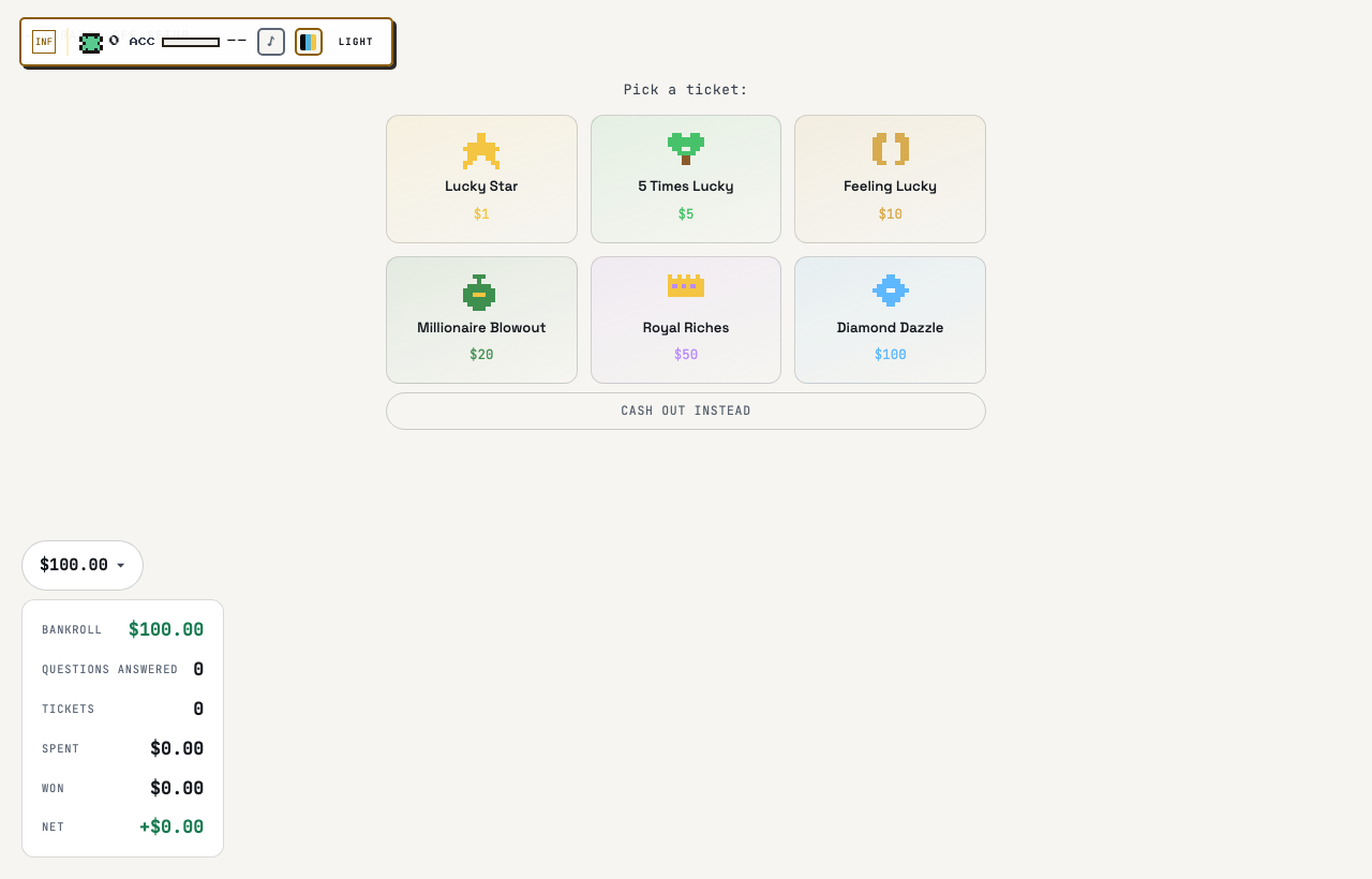
You start with a $100 bankroll and pick a ticket priced at $1, $5, $10, $20, $50, or $100. The ticket flips over to reveal its true prize table before you commit to anything - three outcomes (a $0 tier, a mid tier, and a jackpot tier) with exact fractional odds out of 8 or 16. Real lotteries hide this table; the game shows it to you because reading it is the whole skill.
Before you can scratch, you answer a set of probability questions about the ticket you are holding: expected value, Bayes / conditional probability, no-replacement batch odds, combinatorics, the geometric distribution (expected tickets to first win), and an occasional classic puzzle (Monty Hall, a birthday-problem variant, coupon collector). Then comes the decision stage: buy anywhere from 0 to 10 tickets of this design at this price. Choosing 0 walks away and refunds the ticket price in full - the game still shows what the ticket would have paid, for the record.
This variant runs 13 questions per ticket with no timer - the deepest practice mode. The session ends only when you cash out or your bankroll hits $0.
How scoring works
A ticket that shows multiplier m pays exactly m times the ticket price - the three tiers are $0, a mid prize of 1x or 2x, and a jackpot of 4x, 5x, 6x, or 8x on a normal ticket, or 8x, 10x, or 12x on a rare mispriced one. The $0 tier always covers between 50% and 80% of the probability mass.
70% of generated tickets are fair-ish: expected value at or below 1x the price, a house edge. 30% are hot: EV strictly above 1x, mispriced in the player's favor. The split is constant and is never adjusted based on whether you are winning or losing.
Walking away at the quantity step (choosing 0) refunds your ticket price - a guaranteed EV of exactly 1.0x, better than most tickets in the game.
Compute EV before the buy decision, every time
The flip reveal hands you the full distribution, so EV is one line of arithmetic: multiply each prize by its probability and add. On a $10 ticket showing P($0) = 5/8, P(2x = $20) = 2/8, P(4x = $40) = 1/8: EV = (2/8)($20) + (1/8)($40) = $5.00 + $5.00 = $10.00 - exactly 1.0x, the best a fair-side ticket ever gets. A harsher fair shape like P($0) = 6/8, P(1x = $10) = 1/8, P(5x = $50) = 1/8 gives EV = (1/8)($10) + (1/8)($50) = $7.50, a 25% house edge.
The end-of-session screen states the game's own summary: most tickets pay out about 7/8 of the price - a 12.5% house edge. Any ticket whose EV multiple comes out at or below 1 is a losing or at best break-even bet, and the refund option (buy 0) strictly dominates buying it.
The no-replacement questions are the interview trap
The batch question tells you a ticket came from a batch of N with exactly W winners, and the previous ticket from the batch won nothing. The answer is W/(N-1), not W/N: removing a known non-winner shrinks the pool but leaves all W winners in it. Treating the draws as independent (answering W/N) is the gambler's-fallacy mistake in reverse - here the odds do move, in your favor.
The geometric question is the other classic: if P(win something) = p, the expected number of tickets to the first win is 1/p. A ticket with p = 6/16 takes 16/6, about 2.67 tickets on average - and every one of those tickets still loses money in expectation if EV is below the price.
Thirteen untimed questions is the study mode
The 18-question bank spans six topics in three phrasings each; a 13-question set guarantees every topic and includes 1 to 3 formal-notation questions (P(B|A), E[X], C(n,r), X ~ Geometric(p)). With no clock, read every explanation after checking - each one shows the exact computation, like E[Payout] as the probability-weighted sum or the batch conditional as W/(N-1).
The fixed classics are worth memorizing here since they recur across sessions: switching after a revealed empty panel wins 2/3; three friends drawing from six designs collide with probability 4/9 (via 1 - 5/9); collecting all three of three designs takes E[T] = 3 x (1 + 1/2 + 1/3) = 5.5 tickets on average.
A worked example
Setup: you buy a $10 ticket and the flip reveal shows this exact prize distribution.
Expected value is the probability-weighted sum of the prizes - set up the sum before touching arithmetic.
Carry out the multiplication and add the terms.
Compare EV to the $10 price to get the expected profit and the house edge.
Sample conditional-probability question on the same ticket: given you win something, what is the chance it is the top prize?
Sample geometric question: with this win probability, how many tickets on average until the first win?
At the decision stage, quantity 0 refunds the ticket price outright - compare that guaranteed EV to the ticket's EV.
Common mistakes
• Buying before doing the EV multiplication. The table is face-up - a ticket that pays 7/8 of its price loses you 12.5 cents per dollar in expectation, every time.
• Answering W/N on the batch question. After a non-winner is removed, W winners remain among N-1 tickets: the answer is W/(N-1).
• Sizing up on a fair ticket to chase the jackpot. Quantity multiplies expected loss just as faithfully as expected gain.
• Ignoring the walk-away option. Buying 0 refunds the full price - a guaranteed 1.0x that beats roughly 70% of tickets generated.
• Skipping the explanations. Untimed 13-question mode exists to study the worked solutions; checking an answer and clicking past the shown computation wastes the mode's whole advantage.
Why interviews test this
Expected value over an explicit discrete distribution is the single most common opener in quant interviews - it tests whether you instinctively price a bet instead of reacting to its best case. The follow-ups here mirror real follow-ups: conditional probability without replacement (does the candidate update on removed outcomes?), the geometric distribution (time to first success), and Bayes on nested events.
The deeper lesson interviewers probe is bet selection and sizing: a trader who can compute EV but still takes -EV bets, or who sizes the same regardless of edge, fails the job even if the arithmetic is right. Declining the bet - quantity 0 - is frequently the correct answer, and saying so out loud is a strong interview signal.
Play Scratch-Off (Untimed, 13 Questions) on Outcry
Scratch-Off (Untimed, 13 Questions) is free to play on Outcry, in the Quitters Never Lose section, and every run is timed and scored. Read the guide once, then play Scratch-Off (Untimed, 13 Questions) and check your score against the strategy above. The guide book has a written guide for every other game, and the practice hub and mock assessments put the same skills under a real screen's clock.