Tail Risk Stress Tester

How it works

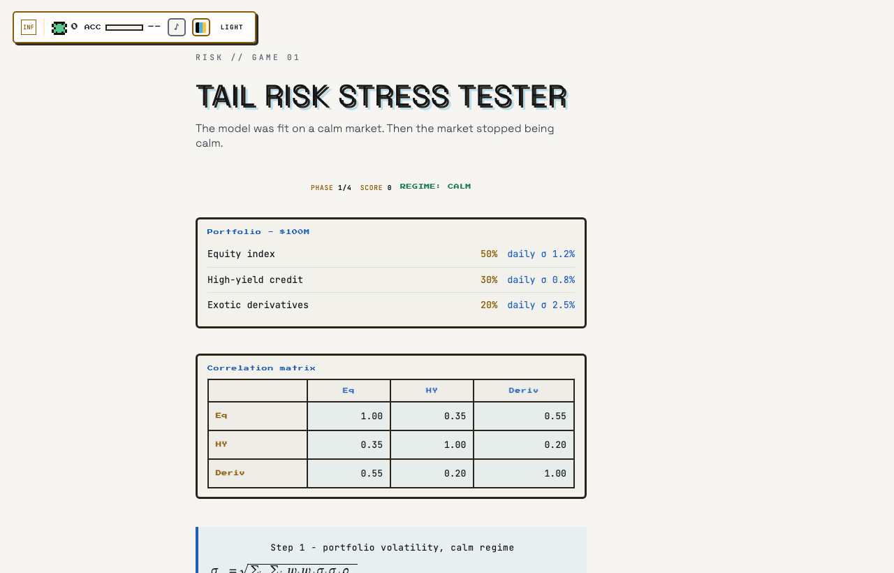
You manage a $100M book with three positions: 50% in an equity index (daily vol 1.2%), 30% in high-yield credit (0.8%), and 20% in exotic derivatives (2.5%). The game runs in four phases. In phase 1 the regime is calm and you compute the portfolio's daily volatility from the given correlation matrix (equity-credit 0.35, equity-derivatives 0.55, credit-derivatives 0.20), entering your answer as a percentage.

In phase 2 the regime flips to stress: every off-diagonal correlation goes to 1.00 while the individual asset vols are unchanged, and you compute the new portfolio volatility. In phase 3 you compute the 99% Expected Shortfall of the stressed book in dollar millions. In phase 4 the game shows what a fat-tailed (Student-t with 4 degrees of freedom) refit does to ES and asks you to pick one of four responses to the situation.

Numeric answers are checked against a tolerance: 0.06 percentage points of volatility for the two vol questions and $0.25M for the ES question. Each question locks after one check, so there are no retries within a run - you can restart the whole stress test at the end.

How scoring works

Points per phase: +2 for the calm portfolio volatility, +3 for the crisis volatility, +3 for the 99% Expected Shortfall in $M, and +2 for choosing the correct hedge, for a maximum of 10 per run.

Volatility answers count as correct within 0.06 percentage points (you type a percent, the game compares it to the exact figure). The ES answer counts within $0.25M. The hedge question has exactly one correct choice: buying deep out-of-the-money index puts.

Each check also records a skill attempt for your readiness profile: the two vol questions record under distributions, the ES question under expected-value, and the hedge choice under optional-stopping.

Portfolio volatility is a double sum you can organize

The formula is sigma_p^2 = sum over i and j of w_i w_j sigma_i sigma_j rho_ij. The clean way to compute it by hand is to first form each position's standalone contribution w_i sigma_i, then square those for the diagonal terms and take pairwise products times correlations for the cross terms. Here the standalone contributions are 0.5 x 1.2% = 0.60%, 0.3 x 0.8% = 0.24%, and 0.2 x 2.5% = 0.50%.

The diagonal terms are 0.60^2 + 0.24^2 + 0.50^2 and each cross pair appears twice, so add 2 x (0.60 x 0.24 x 0.35 + 0.60 x 0.50 x 0.55 + 0.24 x 0.50 x 0.20). Working in percentage units keeps the arithmetic sane; take the square root at the end.

The key sanity check: with correlations below 1, portfolio vol must come out below the plain weighted sum of vols (here 1.34%). The gap between your answer and that weighted sum is the diversification benefit. If your calm answer is at or above 1.34%, you made an arithmetic error.

At rho = 1 the formula collapses - use the shortcut

When every pairwise correlation is 1, the double sum becomes a perfect square: sigma_p = sum of w_i sigma_i, the plain weighted average of the vols. You do not need to redo the matrix computation in phase 2 - just add 0.60% + 0.24% + 0.50% = 1.34%.

This is the deepest fact in the game: the crisis vol jump happens with no change in any single asset's volatility. Only the relationships changed. Diversification is a property of the correlation structure, and in a liquidity vacuum that structure is exactly what disappears - everyone sells everything at once.

Knowing the collapse cold also gives you the phase 1 sanity bound for free: the calm vol must sit strictly between the largest single contribution and the weighted sum.

ES is a formula, not a simulation

For a normal loss distribution, 99% VaR is z_0.99 x sigma with z_0.99 = 2.3263, and Expected Shortfall is ES = sigma x phi(z_alpha) / (1 - alpha), where phi is the standard normal density. At the 99% level phi(2.3263) = 0.02665, so ES = sigma x 0.02665 / 0.01 = sigma x 2.665. Notice that is only slightly above the VaR multiplier of 2.3263 - under a normal, the tail beyond VaR is thin.

Convert to dollars at the end: multiply the ES fraction by the $100M NAV. With the crisis sigma of 1.34%, ES = 1.34% x 2.665 = 3.57%, or $3.57M against a VaR of $3.12M.

The conceptual point the final phase drives home: ES is always at least VaR, and unlike VaR it is subadditive - merging two books can never make ES look better than the sum of the parts. VaR can, which lets a firm hide risk by splitting a book across desks. That property is why regulators moved to ES.

A worked example

Phase 1, calm regime. Standalone contributions: equity 0.5 x 1.2% = 0.60%, credit 0.3 x 0.8% = 0.24%, derivatives 0.2 x 2.5% = 0.50%.

Variance in percent-squared units: diagonal 0.36 + 0.0576 + 0.25 = 0.6676. Cross terms: 2 x (0.60 x 0.24 x 0.35 + 0.60 x 0.50 x 0.55 + 0.24 x 0.50 x 0.20) = 2 x (0.0504 + 0.165 + 0.024) = 0.4788. Total 1.1464, square root 1.07%. Enter 1.07.

Phase 2, crisis. All correlations go to 1, so sigma_p is just the weighted sum: 0.60 + 0.24 + 0.50 = 1.34%. Enter 1.34. That is a roughly 25% jump in portfolio vol with no asset getting riskier, and 99% VaR is now 2.3263 x 1.34% = 3.12% of NAV, about $3.12M - through the $3.00M limit.

Phase 3, shortfall. ES = 1.34% x 0.02665 / 0.01 = 3.57% of NAV = $3.57M. Enter 3.57 (tolerance $0.25M). The average bad day beyond VaR is about 15% worse than the VaR number you were reporting.

Phase 4. The t(4) refit lifts ES by about 40% to roughly $5.0M at the same sigma. The correct action is buying deep out-of-the-money index puts - the only choice that pays off specifically in the tail. Diversifying further fails because correlation convergence is what just broke; sitting inside the VaR limit ignores that VaR says nothing past its own threshold; adding to the position averages into a liquidity vacuum.

Common mistakes

• Forgetting to double the cross terms. Each pair (i, j) appears twice in the double sum. Missing the factor of 2 gives a calm vol that is too low.

• Recomputing the full matrix in the crisis phase. At rho = 1 the answer is just the weighted sum of vols - doing the long computation invites arithmetic slips under time pressure.

• Answering VaR when the game asks for ES. Phase 3 wants sigma x phi(z) / (1 - alpha) in dollars, not z x sigma. The two differ by about 15% at the 99% level, well outside the $0.25M tolerance.

• Mixing units. Vol answers go in as percentages (1.34, not 0.0134); the ES answer goes in as dollar millions (3.57, not a percent). Read the placeholder text.

• Picking further diversification as the hedge. It sounds prudent, but adding more correlated assets when correlations have converged to 1 adds exposure, not protection.

Why interviews test this

"What is wrong with VaR?" is asked in essentially every risk interview, and the strong answer is the one this game trains: VaR is not wrong because it is inaccurate, it is wrong because it is silent about everything past its own threshold, and it is not subadditive, so it can be gamed by splitting books. Follow up with why Basel moved to a 97.5% ES and you are ahead of most candidates.

The correlation-breakdown computation is also a live interview exercise: given weights, vols, and a correlation matrix, compute portfolio vol, then recompute at rho = 1. Interviewers use it to check both the double-sum mechanics and whether you know that diversification is a correlation statement, not an asset-count statement. The fat-tail phase maps to the standard follow-up about why normal-based risk numbers understate crises.