Stochastic Processes · Ruin Walker
Ruin Walker Strategy - Cramér-Lundberg Guide
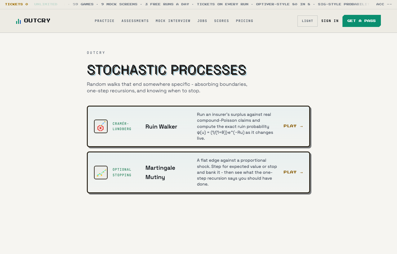
Run an insurance book under the Cramér-Lundberg model - choose your safety loading, answer a closed-form question each period, and try to survive 12 periods without your surplus going negative.
What is a random walk?
A random walk is a stochastic process built by summing independent random steps: X₀ is a starting point, and Xₙ = Xₙ₋₁ + (the n-th step), where each step is drawn from some fixed distribution independent of the others. It is the simplest model of a quantity that accumulates uncertainty over time - a position, a balance, a count - and it is the discrete-time ancestor of nearly every continuous stochastic process used in practice, including Brownian motion, which arises as the limit of a random walk as the step size shrinks and the number of steps grows.
The classic instance is the gambler's ruin problem: a walker starts with some capital and, at each step, wins or loses a fixed amount according to a fixed probability, stopping the moment capital hits zero (ruin) or reaches a target ceiling (success). Even when each individual step has a favorable expected value, the walk can still hit an absorbing lower barrier before it has a chance to compound that edge. Ruin depends on the path the walk takes, on the variance of each step, and on how far away the barrier sits.
A key generalization replaces fixed-size steps with a compound process: capital increases by a steady, deterministic rate but decreases by a random shock process, for example insurance claims arriving at random times and random sizes. This is the Cramér-Lundberg model of ruin theory, and its central result is that the probability of ever being ruined decays exponentially in the starting capital, at a rate called the adjustment coefficient, provided the average rate of increase exceeds the average rate of loss. That exponential decay is the reason a little extra starting capital or a little extra safety margin buys a disproportionate reduction in risk.
Random walks and their ruin probabilities matter well beyond insurance. A trading strategy's account balance, a market maker's inventory, and a hedge fund's drawdown all behave like a random walk with drift, and the same ruin mathematics answers the practical question of how much capital is needed to survive a given strategy at a given confidence level. The gambler's ruin framework is also a standard building block for pricing barrier options and for reasoning about hitting times and absorbing boundaries in any process built from repeated random increments.
How it works
You run an insurance book. Your surplus starts at 20 ticks and you have a $100 bankroll. Before the run you choose two things: a safety loading θ from the options 10%, 25%, 50%, or 100%, and a stake per unit of surplus from $1, $2, $5, or $10. The loading sets your premium: the book collects (1+θ)·λ·μ ticks per period, with claim rate λ = 1 per period and mean claim size μ = 5 ticks.
Each of the 12 periods works the same way. First you are asked one question drawn from a procedural bank of eight Cramér-Lundberg quantities - the ruin probability ψ(u) from the current surplus, ψ(0), the adjustment coefficient R, the premium rate c, Lundberg's bound e^(-Ru), the surplus needed to hit a target ruin probability, expected claims per period, or the net drift. The question uses the live surplus and your chosen θ, so you cannot recycle last period's answer. After checking your answer you run the period: a Poisson(λ) number of claims arrives, each claim is exponentially distributed with mean μ, premium is added, claims are subtracted, and the new surplus appears.
Ruin is absorbing: the moment surplus goes below zero the run ends, no matter how it happened. Survive all 12 periods and the book closes solvent. From period 1 onward, any period where you have not yet checked the question you can also close the book early and cash out at the current surplus.
How scoring works
Your profit and loss is (final surplus - 20) x your chosen stake per unit. The final bankroll is $100 plus that P&L.
The leaderboard ranks rounded profit in dollars. Everyone starts from the same $100, so this compares judgement across different stake sizes.
The per-period questions are graded against the exact closed forms with a stated tolerance (for example 2 percentage points on probability questions, 0.005 on R). Probability answers accept either percent form like 36% or decimal form like 0.36. Getting a question wrong does not end the run or cost surplus - the reveal shows the correct value and explanation, then the period runs regardless.
The model: surplus as a compound Poisson process
The Cramér-Lundberg model describes an insurer's surplus as U(t) = u + c·t - S(t): a starting cushion u, a deterministic premium stream at rate c, minus a compound Poisson claims process S(t). Claims arrive at Poisson rate λ, and each claim size is drawn independently - here from an exponential distribution with mean μ. Ruin means the surplus ever dips below zero.
The first thing to check in any such model is the net profit condition: c > λμ, equivalently θ = c/(λμ) - 1 > 0. In this game expected claims per period are λμ = 5 ticks, so a loading of θ = 25% means you collect 6.25 ticks of premium against 5 ticks of expected claims - a positive drift of θλμ = 1.25 ticks per period. Positive drift is necessary for survival but not sufficient: variance around that drift is what kills books, because one bad Poisson draw can stack several large exponential claims into a single period.
The mean tells you which way you drift. Ruin probability is governed by the tail of the fluctuations, which is why the formula carries an exponential decay rate on top of the drift.
The adjustment coefficient and the exact ruin formula
The adjustment coefficient R is the exponential decay rate of ruin risk in the initial surplus. For exponential claims it has the clean closed form R = θ / ((1+θ)μ), and the ruin probability is exact: ψ(u) = (1/(1+θ))·e^(-Ru). For a general claim distribution you lose the exact formula but keep Lundberg's inequality, ψ(u) ≤ e^(-Ru), which is why the game sometimes asks for the bound separately - the bound holds for any claim size distribution, and for exponential claims the exact answer is smaller by exactly the factor 1/(1+θ).
Two facts anchor every question in the bank. First, ψ(0) = 1/(1+θ) exactly: starting with zero surplus, the book still survives with positive probability as long as the loading is positive, because the premium stream can outrun claims. Second, each extra tick of surplus multiplies the ruin probability by e^(-R) - safety compounds exponentially in u. Inverting that gives the required-surplus question: to push ψ down to a target, solve u = ln[(1/(1+θ))/target] / R.
Precompute R the moment you choose θ, because it never changes during the run. At θ = 25% and μ = 5, R = 0.25/(1.25·5) = 0.04. At θ = 100%, R = 1/(2·5) = 0.10. Then every ψ(u) question is one exponential away, and every required-surplus question is one logarithm away.
Choosing θ and stake: risk of ruin versus expected profit
Higher θ makes the book strictly safer: it raises the drift, raises R, and shrinks ψ(u) at every surplus level. From the starting surplus of u = 20, the exact ruin probabilities are ψ(20) = (1/1.1)·e^(-0.1/(1.1·5)·20) ≈ 63% at θ = 10%, about 36% at θ = 25%, about 26% at θ = 50%, and about 7% at θ = 100%. The θ = 10% book is more likely than not to be ruined eventually - within 12 periods the risk is lower than the eventual figure, but the ranking across loadings is the same.
Higher θ also raises expected profit: drift is θλμ per period, so θ = 100% earns 5 ticks per period in expectation versus 0.5 at θ = 10%. In this game there is no penalty for charging more - unlike a real market, demand does not fall when premium rises - so a high loading dominates on both safety and expected P&L. The interesting decision is the stake: stake multiplies both your P&L and your variance, and pairs of (θ, stake) let you dial total risk.
The cash-out option is worth understanding through the drift lens. With positive drift, every additional period has positive expected value, but it also carries ruin risk that wipes the whole position. Cashing out early after a lucky run locks in surplus above theory; the model itself says the long-run trend is up, so cashing out trades expected value for lower variance.
A worked example
Setup: current parameters and question - find ψ(u), the ruin probability from here.
Adjustment coefficient - matches the R tile the HUD displays throughout.
The prefactor of the exact ruin formula - also equal to ψ(0), the ruin probability starting from zero surplus.
Evaluate the exponent and its value.
Combine for the exact ruin probability.
Grading tolerance is 2 percentage points, and two sanity checks confirm the answer's range.
Common mistakes
• Forgetting the 1/(1+θ) prefactor and answering e^(-Ru) - that is Lundberg's bound. For exponential claims the exact answer is always smaller by that factor.
• Answering ψ(0) = 100%. With positive loading a book starting from zero surplus survives with probability θ/(1+θ) - the premium margin alone can outrun claims.
• Using the starting surplus of 20 instead of the current surplus. Questions are drawn off the live state of the book, and surplus enters through the exponential, so this error compounds fast.
• Confusing premium c = (1+θ)λμ with net drift c - λμ = θλμ. One is what you collect, the other is what you expect to keep.
• Treating a survived period as evidence the book is safe. Ruin is absorbing and the per-period claim total has an exponential tail - one heavy period can erase many good ones, which is what R quantifies.
Why interviews test this
The Cramér-Lundberg model is the canonical first model in actuarial exams and insurance-flavored quant interviews: expect to be asked for the net profit condition, the adjustment coefficient, and Lundberg's inequality, and to explain why ruin probability decays exponentially in initial capital.
The same mathematics shows up outside insurance as risk of ruin for a trading book or a bankroll: a positive-drift process with heavy-tailed downside still has nonzero ruin probability, and the exponential-in-capital decay is the standard answer to 'how much capital do I need for a target survival probability'. Interviewers also like the ψ(0) = 1/(1+θ) fact as a quick check of whether you understand the formula.
Play Ruin Walker on Outcry
Ruin Walker is free to play on Outcry, in the Stochastic Processes section, and every run is timed and scored. Read the guide once, then play Ruin Walker and check your score against the strategy above. The guide book has a written guide for every other game, and the practice hub and mock assessments put the same skills under a real screen's clock.