Actuarial Lab · Loss Triangle Labyrinth
Loss Triangle Guide - Chain Ladder and BF
Develop a run-off triangle with chain ladder link ratios, set the total reserve, and know when to switch to Bornhuetter-Ferguson.
What is a loss triangle / chain-ladder reserving?
An insurer collects a premium today for a promise to pay claims that may not be fully known, or fully paid, for years afterward - a car accident, a liability suit, or a workers' comp injury can all take a long time to settle in full. Estimating how much money to set aside today for claims that have already happened but are not yet fully paid is called reserving, and getting it wrong in either direction is costly: reserve too little and solvency is threatened when the bills come due; reserve too much and capital sits idle that could have been put to use.
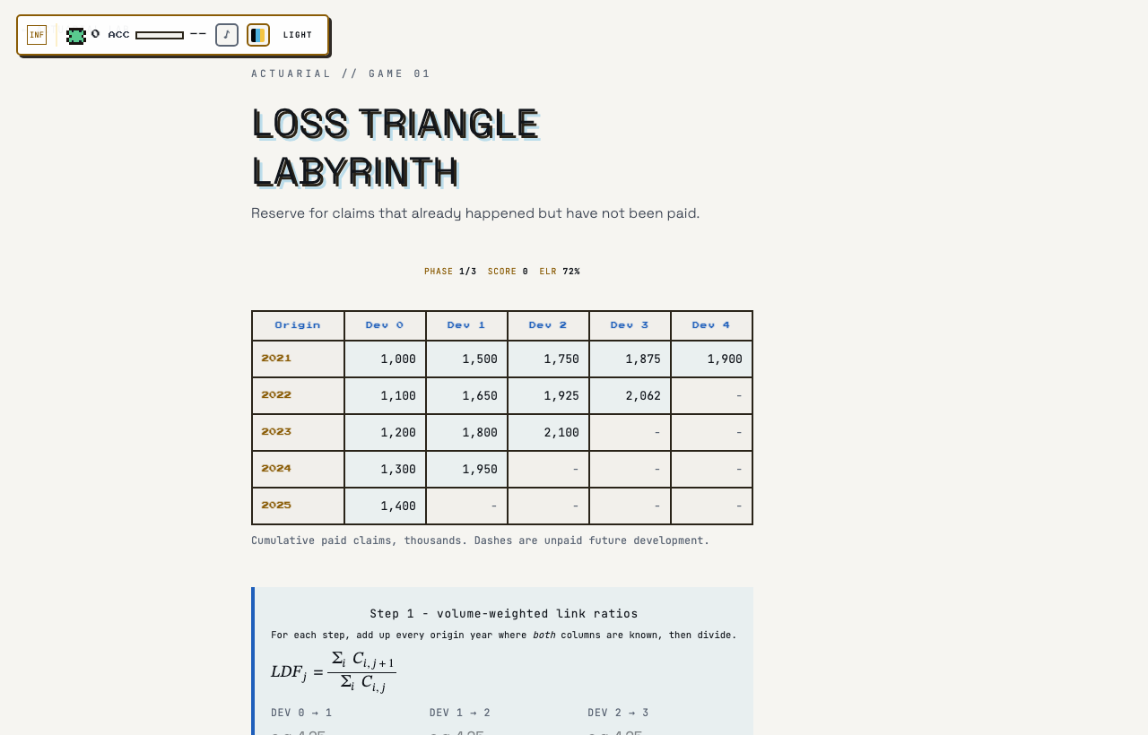
The loss triangle is the standard way this data is organized. Claims are laid out by origin year (when the policy or accident occurred) down the rows, and by development period (how many years since origin the claims have had to accumulate) across the columns. Because older origin years have had more time to develop, the triangle is fully populated in one corner and increasingly empty toward the other, forming the triangular shape the method is named for - and the empty corner is exactly the unknown future the actuary has to estimate.
The chain-ladder method assumes that the pattern by which claims grow from one development period to the next is stable across origin years, regardless of how large or small a given year's claims happen to be so far. It estimates a link ratio (or loss development factor) for each development step - typically a ratio of sums across all years with data at both ages, which weights larger, more credible years more heavily than small or noisy ones - and then chains those ratios together to project every immature year's current claims out to an expected ultimate value. It's one of the oldest reserving techniques in practice because it requires nothing more than the triangle itself and this one stability assumption.
That stability assumption breaks down for very immature years, where a small amount of noisy early data gets multiplied by a large development factor and any randomness in that first number is amplified straight into the final reserve. Bornhuetter-Ferguson is the standard remedy: instead of scaling up the observed claims, it blends the chain-ladder projection with an independent, outside estimate of ultimate losses - typically premium times an expected loss ratio - weighting each by how much of the ultimate loss the triangle would already expect to have seen by now. The less developed a year is, the more the estimate leans on the outside expectation.
Reserve estimates are one of the largest single sources of volatility in an insurer's reported earnings and solvency position, which is why reserving methodology sits at the center of actuarial practice and regulatory review. The underlying idea - blend an observed trend with an independent prior estimate, weighted by how much you trust the data seen so far - recurs throughout actuarial work under the name credibility theory.
How it works
You are handed a run-off triangle of cumulative paid claims in thousands: five origin years (2021 to 2025) as rows, development years as columns. 2021 is fully developed through five columns (1000, 1500, 1750, 1875, 1900); each later year has one fewer entry, down to 2025 with a single figure of 1400. The dashes in the lower-right are money you owe but have not paid, and the game is about estimating it.
Phase 1 asks for the four volume-weighted link ratios, one per development step: for each step, sum the later column across every origin year where both columns are known, sum the earlier column over the same years, and divide. Each ratio is checked within 0.01. Phase 2 asks for the total chain ladder reserve: project each origin year's latest figure to ultimate using the product of remaining link ratios, subtract what is already paid, and sum across years (tolerance 40).
Phase 3 focuses on 2025, the year with one data point and a cumulative development factor near 1.9. You choose a method - stay with chain ladder or switch to Bornhuetter-Ferguson - and then compute the 2025 reserve given a premium of 2,600 and an expected loss ratio of 72%. The value is checked against the BF answer within 40. All answers lock after one check; you can rerun the triangle at the end.
How scoring works
Phase 1: +1 point per link ratio within 0.01, four available. Phase 2: +2 points for the total reserve within 40. Phase 3: +1 point for choosing Bornhuetter-Ferguson (the only choice scored as correct) and +2 points for the reserve value within 40 of the BF figure. Maximum 9 per run.
The value check in phase 3 is against the BF reserve regardless of which method you selected, so picking chain ladder and entering the chain ladder number scores zero on both counts.
Checks record skill attempts under distributions (link ratios), expected-value (both reserve figures), and selection-bias (the method choice).
Volume-weighted link ratios
The chain ladder estimator for each development step is LDF_j = sum of C_(i,j+1) over sum of C_(i,j), taken only across origin years where both columns exist. It is a ratio of sums, not an average of ratios: a large mature year carries more weight than a tiny immature one, which is the standard estimator because it weights each year by its exposure.
Mechanically, for step 0 to 1 you use four origin years (2021 through 2024 all have both columns), for step 1 to 2 three years, and so on down to a single year for the last step. Write the two column sums before dividing - the discipline prevents the classic error of including an origin year whose later column does not exist.
This triangle is built to develop cleanly: the ratios come out at 1.5, about 1.1667, about 1.0713, and about 1.0133. Ratios should shrink toward 1 as development matures; if yours do not decline monotonically, recheck which rows you summed.
From ratios to reserves via CDFs
The cumulative development factor for an origin year is the product of every link ratio from its current development age to ultimate. 2021 is at ultimate (CDF 1, reserve zero); 2022 needs only the last ratio; 2025 needs all four multiplied together, about 1.90.
Each year's ultimate is its latest cumulative figure times its CDF, and its reserve is ultimate minus latest - the reserve is only what has not been paid yet, never the whole ultimate. Sum the per-year reserves for the total. A useful check: the reserve should be dominated by the youngest years, since they have the most development remaining.
The 40-tolerance on the total is tight enough that you should carry the ratios to four decimals through the CDF products rather than rounding each ratio to two places first.
Why the thin year breaks chain ladder, and what BF does instead
2025 has exactly one payment, 1,400, and a CDF near 1.9. Chain ladder multiplies that single noisy figure by almost 1.9, so any randomness in the first payment is amplified straight into the reserve - this is the leverage problem, and it is the one situation where chain ladder is the fragile choice.
Bornhuetter-Ferguson sidesteps it by never scaling the actual claims up. The BF reserve is (1 - 1/CDF) x premium x expected loss ratio: apply the undeveloped share of the pattern to an independent a-priori expectation instead of to the observed figure. An erratic early payment cannot dominate the estimate.
BF is exactly a credibility blend: Z x chain ladder + (1 - Z) x a-priori, with Z = 1/CDF, the share of losses you would expect to have paid by now. It always sits between the two estimates and leans on the a-priori whenever the year is barely developed - which is the phase 3 situation by construction.
A worked example
Phase 1 setup: the volume-weighted link ratio for a development step is the sum of the later column over the sum of the earlier column, across origin years where both are known.
Compute all four link ratios from the triangle's column sums.
Phase 2: chain each year's remaining link ratios together to get its cumulative development factor (CDF).
The reserve formula: project the latest paid figure to ultimate with the CDF, then subtract what is already paid.
Apply it to 2022 through 2024.
Apply it to 2025 (the year with a single data point and the largest CDF), then sum every year's reserve for the total. Enter about 1,987.
Phase 3: since 2025 is barely developed, switch to Bornhuetter-Ferguson, which applies the undeveloped share of the pattern to an a-priori expectation instead of scaling the noisy observed figure.
Substitute 2025's CDF, premium, and expected loss ratio. Enter about 887, well below chain ladder's roughly 1,260.
Common mistakes
• Averaging the individual year-over-year ratios instead of taking the ratio of column sums. The volume-weighted estimator is sums first, then divide; the simple average lets a small year distort the factor.
• Including an origin year in a link ratio when its later column does not exist yet. Only rows with both columns known enter the sums.
• Reporting ultimates instead of reserves. The reserve is ultimate minus latest paid - forgetting the subtraction roughly doubles your phase 2 answer.
• Rounding link ratios to two decimals before multiplying into CDFs. The compounding pushes the total outside the 40 tolerance; keep four decimals.
• Entering the chain ladder figure in phase 3. The value check is against the BF reserve of about 887, and staying with chain ladder also forfeits the method point.
Why interviews test this
Every P&C reserving interview starts with a triangle, and this is the standard sequence: compute volume-weighted link ratios, chain the CDFs, state the reserve as ultimate minus paid. Getting the ratio-of-sums estimator right (and saying why it beats a simple average) is the baseline; the differentiator is knowing the one situation where chain ladder blows up.
"When would you not use chain ladder?" is the classic follow-up, and the answer this game drills is the one interviewers want: an immature year with high leverage, where you switch to Bornhuetter-Ferguson and can explain it as a credibility weighting between the development-based estimate and an a-priori expectation, with Z = 1/CDF. This material maps directly to the reserving portions of the actuarial exam track and to case questions at consulting and insurance employers.
Play Loss Triangle Labyrinth on Outcry
Loss Triangle Labyrinth is free to play on Outcry, in the Actuarial Lab section, and every run is timed and scored. Read the guide once, then play Loss Triangle Labyrinth and check your score against the strategy above. The guide book has a written guide for every other game, and the practice hub and mock assessments put the same skills under a real screen's clock.