Gradient Lab · Lagrange Optimizer
Lagrange Optimizer Guide - Constrained Optimization
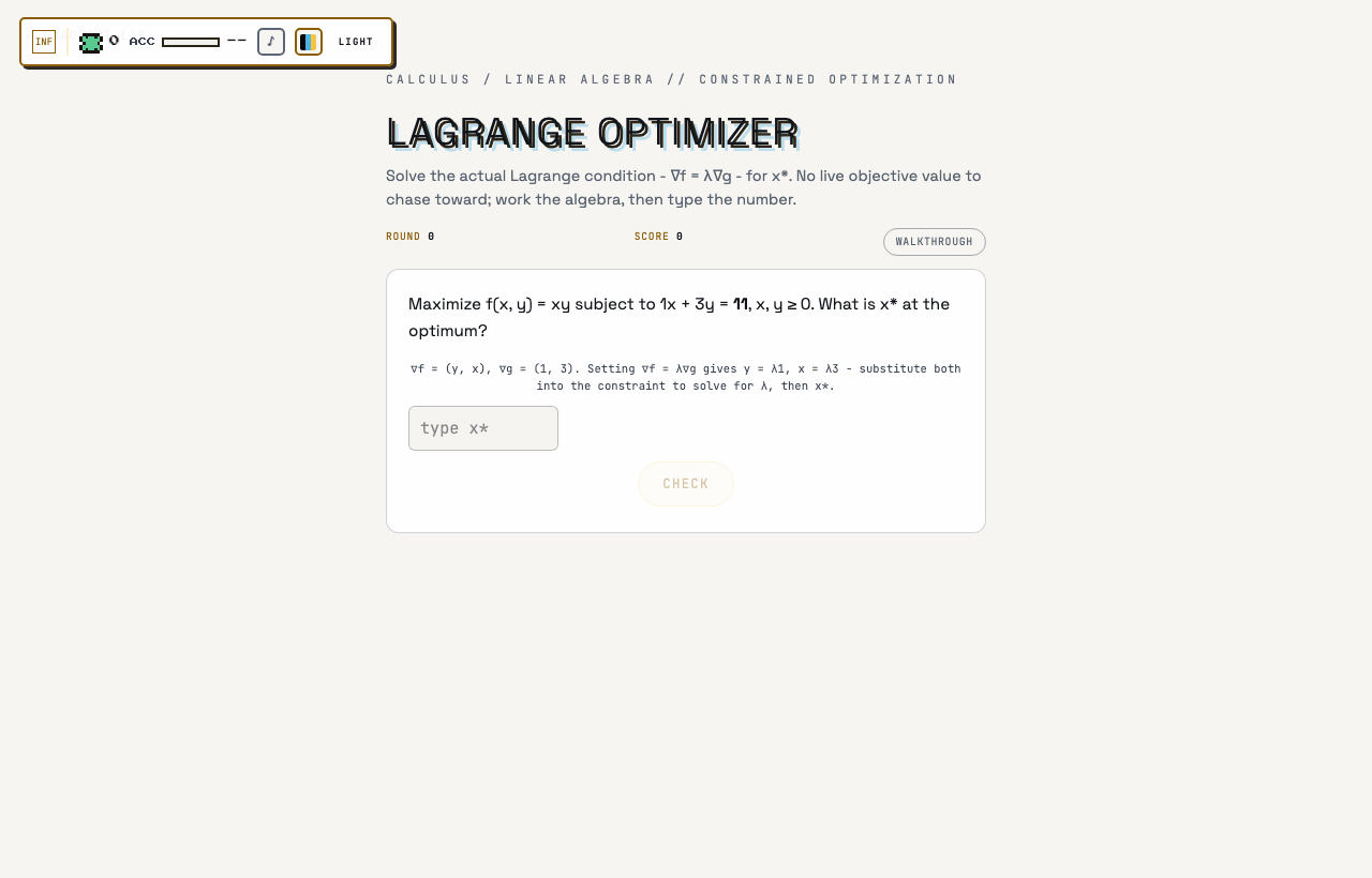
Maximize xy on a budget line ax + by = k by solving the Lagrange condition ∇f = λ∇g for x* with nothing but the algebra - there is no live readout to chase.
What is Lagrangian optimization?
Lagrangian optimization is the standard method for maximizing or minimizing a function subject to equality constraints. Given an objective f(x) and a constraint g(x) = c, the method forms the Lagrangian L(x, λ) = f(x) - λ(g(x) - c) and looks for points where its gradient with respect to both x and λ vanishes. Setting ∂L/∂x = 0 recovers the condition ∇f = λ∇g, and setting ∂L/∂λ = 0 recovers the original constraint - so solving the Lagrangian's stationarity conditions solves the constrained problem directly, without ever having to eliminate a variable by hand.
The geometric idea behind ∇f = λ∇g is tangency. Picture the level curves of f as contour lines and the constraint g(x) = c as a fixed path through them. At any point where the path crosses a contour line at an angle, you could slide along the path to a better contour, so that point cannot be optimal. The optimum can only occur where the path is tangent to a contour line - where the two gradients, both perpendicular to their respective curves, point in the same or opposite direction. That parallelism is exactly what ∇f = λ∇g states.
The multiplier λ is the shadow price of the constraint, equal to the rate at which the optimal value of f changes as the constraint level c is relaxed: λ = d(optimal f)/dc. This interpretation extends naturally to inequality constraints through the Karush-Kuhn-Tucker conditions, where each multiplier measures how much the objective would improve if that particular constraint were loosened, and a multiplier of zero means the constraint is not binding at the optimum.
Constrained optimization of this kind is everywhere in quantitative finance. Mean-variance portfolio optimization is a Lagrangian problem - minimize portfolio variance subject to a target expected return and a full-investment constraint - and its multipliers are what produce the efficient frontier. Utility maximization under a budget constraint, maximum-entropy modeling under moment constraints, and risk-parity allocation under a leverage constraint all reduce to the same gradient-alignment condition. Recognizing a problem as 'optimize this, subject to that' and reaching for ∇f = λ∇g is one of the most transferable pieces of mathematical machinery in the field.
How it works
Each round generates a fresh problem: maximize f(x, y) = xy subject to ax + by = k with x, y ≥ 0, where a and b are random integers from 1 to 4 and k is a random integer from 6 to 21. You are asked for x* at the optimum and must type the number - there is no live objective readout to converge on visually.
The hint on screen sets up the method: ∇f = (y, x) and ∇g = (a, b), so the Lagrange condition ∇f = λ∇g gives y = λa and x = λb. Substituting both into the constraint yields a(λb) + b(λa) = k, so λ = k/(2ab), and then x* = λb and y* = λa.
After you check, the reveal walks the full solution: λ, x*, y*, a numerical check that ax* + by* ≈ k, and the maximum value of xy. Press next round for a new (a, b, k).
How scoring works
Your typed x* is graded within a tolerance of max(0.01, 1% of x*). A correct answer adds 1 to score; every checked answer adds 1 to rounds. There are no partial points and no timer.
The geometry: gradients must align on the constraint
At a constrained optimum, the level curve of the objective is tangent to the constraint set - if it crossed the constraint, you could slide along the constraint and improve. Tangency means the normals line up: ∇f = λ∇g. The multiplier λ is the proportionality factor, and economically it is the shadow price - the rate at which the optimal value grows per unit of extra k.
For this game's family, ∇f = (y, x) points perpendicular to the hyperbola xy = constant, and ∇g = (a, b) is the fixed normal of the budget line. The condition (y, x) = λ(a, b) says the optimal point is where a hyperbola just kisses the line. Everything after that is substitution.
Notice the cross-symmetry in the result: x* = λb and y* = λa - x* picks up b, the coefficient on the other variable. Working through why (y matches a because ∂f/∂x = y sits opposite the a-slot) inoculates you against the most common slip in this game.
The closed form and the equal-split interpretation
Carry the algebra to the end once and you never redo it: λ = k/(2ab), x* = λb = k/(2a), y* = λa = k/(2b). So the optimum spends exactly half the budget on each term: ax* = k/2 and by* = k/2. For maximizing a product under a linear budget, splitting the budget equally across the terms is the general pattern - the same result AM-GM gives.
That gives you a five-second solve for any round: x* = k/(2a). If a = 3 and k = 18, x* = 3. The maximum value is x*·y* = k²/(4ab) if you want the sanity check the reveal shows.
The AM-GM route is worth knowing as the cross-check: with u = ax and v = by, u + v = k fixed, and xy = uv/(ab) is maximized when u = v = k/2. Two independent methods landing on the same number is exactly the kind of verification interviewers like to see.
Where Lagrange multipliers earn their keep
The method generalizes far beyond this toy: any smooth objective with equality constraints yields stationarity of the Lagrangian L = f - λ(g - k). In quant work this is portfolio optimization (maximize expected return subject to a risk budget and full investment - the classic mean-variance solution is a Lagrange computation), utility maximization under a budget, and maximum entropy distributions under moment constraints.
The multiplier itself is often the deliverable: λ = ∂(optimal value)/∂k tells you what one more unit of budget or risk is worth. In this game, the optimal value is k²/(4ab), and differentiating with respect to k gives k/(2ab) - exactly the λ you computed. That identity is a favorite follow-up question.
Also keep the boundary caveat in mind: Lagrange finds interior tangency points. Here the constraint x, y ≥ 0 is slack at the optimum (both come out strictly positive), so the tangency point is the answer - but in general you must check corner solutions too.
A worked example
Setup: maximize xy on the budget line, with x, y ≥ 0.
Lagrange condition: the gradients must be parallel.
Substitute into the constraint to solve for λ - matches the general closed form λ = k/(2ab).
Read off the optimum. Answer: x* = 3.
Grading tolerance is 1% of the answer.
Verify: the budget is spent exactly, split evenly, and gives the claimed maximum value.
Nudge test confirms tangency: a nearby point on the same budget line scores lower.
Common mistakes
• Swapping the coefficients: writing x* = λa instead of x* = λb. Because ∇f = (y, x) crosses the variables, x pairs with b - the equal-split form x* = k/(2a) is the safest way to remember it.
• Setting ∇f = ∇g without λ - solving y = a, x = b. That point almost never lies on the constraint; the multiplier is what scales the gradient direction to reach it.
• Answering the maximum value of xy, or y*, when the question asks for x*. Read what is asked before typing.
• Splitting x and y equally instead of splitting the budget equally. The optimum has ax* = by* = k/2; x* = y* only when a = b.
• Ignoring the check the reveal offers: if a·(your x*) is not close to k/2, you slipped somewhere. Verification against the constraint is free and catches sign and swap errors instantly.
Why interviews test this
Constrained optimization is the backbone of the quant-research canon: mean-variance portfolios, maximum likelihood under constraints, and utility maximization are all Lagrange computations, and interviews regularly ask a small closed-form instance exactly like this game's - maximize a product or a log-sum under a linear budget.
The two follow-ups to prepare: interpret λ as a shadow price (the derivative of the optimal value with respect to the constraint level), and reproduce the answer by a second route such as AM-GM or direct substitution of y = (k - ax)/b followed by one-variable calculus. Interviewers use the second route to separate memorized formulas from understanding.
Play Lagrange Optimizer on Outcry
Lagrange Optimizer is free to play on Outcry, in the Gradient Lab section, and every run is timed and scored. Read the guide once, then play Lagrange Optimizer and check your score against the strategy above. The guide book has a written guide for every other game, and the practice hub and mock assessments put the same skills under a real screen's clock.