Statistics Lab · Crack the Bot

Crack the Bot Strategy Guide

Infer the hidden rule driving an algorithmic trader by running real regressions on its tape - and learn to say 'there is no rule' when the data says so.

Crack the Bot in play on Outcry — Crack the Bot, in play.

What is statistical significance testing?

Whenever a pattern turns up in data, the first question is whether it reflects something real or is just what randomness produces on its own. A hypothesis test answers this formally. You state a null hypothesis - typically 'there is no effect, no relationship, no rule' - and compute a test statistic, such as a regression coefficient's t-statistic, which is the estimated effect divided by its standard error. The p-value is the probability of seeing a result at least this extreme if the null hypothesis were actually true. A small p-value is evidence against the null, not proof of the alternative.

The standard error in that ratio shrinks roughly with the square root of the sample size, so the same underlying effect produces a weak, inconclusive statistic on a small sample and a strong, obvious one on a large sample. This is why an estimate's size alone tells you little - a large slope on ten observations can be indistinguishable from noise, while a small slope on ten thousand observations can be extremely unlikely to be chance. Reading significance means looking at the statistic as well as the point estimate.

A separate problem appears the moment you run more than one test: the multiple-comparisons problem. If you check twenty independent hypotheses at a 5% significance threshold, and none of them are real, you should still expect roughly one to look significant by chance alone, because a 5% threshold is defined to produce false positives 5% of the time per test. Corrections such as Bonferroni's - dividing the significance threshold by the number of tests - restore the intended overall false-positive rate. This is the same reasoning that makes clinical trials, genomic screens, and A/B tests all report corrected significance levels.

A further way a test can mislead has nothing to do with sample size or multiplicity: omitted-variable bias, also called confounding. If the variable you are testing is itself correlated with some other, unmeasured driver of the outcome, a regression that leaves that driver out will attribute part of its effect to the variable that happens to be standing in for it. The fix is to control for the suspected confound directly and see whether the original relationship survives - if it collapses once the real driver is included, the original result was borrowed significance.

Telling a real signal from noise, and refusing to be fooled by a search over many candidate explanations, is the daily work of quantitative research, epidemiology, and policy evaluation alike - fields where the cost of calling noise a discovery is measured in wasted capital, failed treatments, or bad policy.

How it works

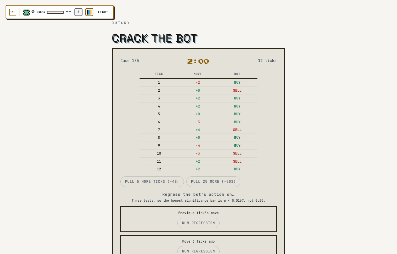
You face five cases, one at a time. In each case a bot trades against a random price tape, and a hidden rule drives its BUY/SELL decisions: momentum (follows the last move), mean reversion (fades the last move), a 3-tick delayed reaction, trend-following on the 5-tick average, or no rule at all. The rule only fires part of the time - the fire rate drops from 100% in case 1 to 75% in case 4, and the final case is pure noise - so the signal gets buried deeper in randomness as you progress.

Each case gives you 12 ticks of tape for free and a 2-minute clock. You can pull 5 or 25 more ticks, but every 5 ticks costs 4 seconds off the clock, so more data costs time. Your main tool is regression: you can regress the bot's action on any of three candidate predictors - the previous tick's move, the move 3 ticks ago, or the average of the last 5 moves - and read back the slope, t-statistic, p-value, and sample size. A confounder-check panel also lets you pick a suspect predictor X, control for a second predictor Z, and predict whether the naive slope shrinks, grows, or holds once Z is in the model.

When you commit to a rule, you must prove it by calling the bot's next 3 moves. If you call 'no rule', there is nothing to predict - the call itself is the answer, and it is right only when the case truly has no rule. Pulling new ticks wipes your existing regression results, since old estimates no longer describe the visible sample.

How scoring works

Each case scores 0 if your rule call is wrong, and otherwise: 100 base points, plus a speed bonus of up to 50 (time remaining as a fraction of the 2-minute clock, times 50), plus a data bonus of max(0, 40 minus the number of extra ticks pulled beyond the free 12), plus 10 points per correct move prediction (up to 3).

Running out of time closes the case at 0. Your total across all five cases is the leaderboard score, and the final banner shows a win at 300 or more points.

Judge by the t-stat

A regression slope tells you the direction and size of an association; the t-statistic tells you whether it could plausibly be zero. The t-stat is the slope divided by its standard error, and the standard error shrinks like 1 over the square root of the sample size. So a slope of 0.1 on 15 observations and a slope of 0.1 on 150 observations are completely different pieces of evidence. In this game the p-value is computed from the t-stat via the normal distribution, and anything driven by a real rule at a decent fire rate will push t well past 2 once you have enough ticks.

The practical habit: never call a rule off a slope alone. Look at n first, then t. With only the 12 free ticks, even a bot on a 100% fire rate can produce lukewarm t-stats because the predictors need lag history (lag1 loses 1 observation, lag3 loses 3, ma5 loses 5). A borderline t around 1.5 to 2 on a small sample is an argument for pulling more ticks.

Mean reversion shows up as a significantly negative slope on the previous tick's move, momentum as a significantly positive one. Sign matters as much as significance: the predictors map to hypotheses, but a negative coefficient on lag1 points at reversion even though lag1 is labelled as the momentum test.

Bonferroni and the no-rule case

You run three tests per case, so a naive p < 0.05 bar gives roughly a 14% chance that at least one predictor looks significant on pure noise. That is the multiple-comparisons trap, and it is why the game displays the corrected threshold as 0.05 divided by 3, about 0.0167. Any p-value between 0.0167 and 0.05 is the zone where noise most often passes for signal.

The final case has no rule at all, and it scores like a win because refusing to trade a false signal is the hardest call. On that case, expect one of the three regressions to occasionally flirt with p < 0.05 - that is what a 1-in-3 false-positive machine does. If nothing survives the Bonferroni bar after a healthy pull of extra ticks, call random and take the points.

This is also the general interview lesson: significance thresholds are per-test guarantees. The more hypotheses you screen, the stronger each individual result needs to be. Correct for the search, or the search will manufacture discoveries for you.

Use the confounder check to break ties

The three predictors are mechanically correlated: the 5-tick average's window contains both the previous move and the 3-tick lag. So when the bot is a trend follower, the lag1 regression can come back significant purely because lag1 rides along with ma5. That is omitted-variable bias: the naive slope on X absorbs beta_Z times the auxiliary slope of Z on X.

The game lets you test this directly. Pick your suspect X, control for a rival Z, and see whether the partial coefficient on X survives. If the true driver is Z, the partial slope on X collapses toward zero while Z stays hot; if X is the real driver, controlling for Z barely moves it. The panel even reconstructs the bias identity for you - naive minus partial equals beta_Z(partial) times the aux slope - so you can watch the arithmetic close.

Tactically, run all three naive regressions first, and whenever two predictors both clear the bar, run the multi-regression before calling. Two significant naive slopes almost always means one true driver plus one passenger, and the partial regression tells you which is which.

A worked example

Case 4 is the trend bot at a 75% fire rate. Pulling 25 extra ticks brings the visible sample to:
$n = 12 + 25 = 37 \text{ ticks}$
Regressing the bot's action on each candidate predictor returns:
$\beta_{\text{lag1}}=0.21,\ t=2.1,\ p=0.036 \qquad \beta_{\text{lag3}}=0.08,\ t=0.8,\ p=0.42 \qquad \beta_{\text{ma5}}=0.55,\ t=3.4,\ p=0.0007$
With three simultaneous tests, the honest significance bar is Bonferroni-corrected:
$\alpha_{\text{corrected}} = \frac{0.05}{3} \approx 0.0167$
Only ma5 clears the corrected bar. lag1's p = 0.036 passes the naive 0.05 cut but fails the corrected one, and lag3 is nowhere close:
$p_{\text{ma5}} = 0.0007 \ <\ 0.0167 \ <\ p_{\text{lag1}} = 0.036 \ <\ 0.05, \qquad p_{\text{lag3}} = 0.42$
Because ma5's window contains lag1, run the confounder check: control X = lag1 for Z = ma5. The partial slope on lag1 collapses toward zero while ma5 stays strong - confirming ma5 is the true driver:
$\beta_{\text{lag1}}^{\text{partial}} \approx 0.04,\quad t \approx 0.4 \qquad \left(\text{down from } \beta_{\text{lag1}}=0.21,\ t=2.1\right)$
Call the rule 'trend', then predict the next 3 moves from the sign of the average of the last 5 visible changes. At a 75% fire rate most predictions land, each worth 10 points on top of the 100-point base plus speed and data bonuses:
$\text{score} = 100 + \text{speed} + \text{data} + 10\times(\text{correct moves},\ \le 3)$

Common mistakes

• Locking in off the free 12 ticks. The lagged predictors eat into your usable sample, and small-n t-stats are unstable - a 4-second cost for 5 more ticks is almost always worth it on the noisier cases.

• Treating p < 0.05 as the bar. With three simultaneous tests the honest threshold is 0.0167, and the gap between them is exactly where the random case will trick you.

• Calling the rule with the wrong sign in mind. A significantly negative slope on the previous move means reversion. Read the direction as well as the significance.

• Ignoring the confounder check when two predictors light up. The overlap between ma5 and the lags means one of them is usually a passenger; the partial regression is a cheap tiebreak.

• Refusing to ever call 'no rule'. The random case pays the full 100-plus base like any other correct call, and forcing a rule onto noise scores zero.

Why interviews test this

This game is a compressed version of the signal-research loop that quant research and econ-consulting interviews probe constantly: given noisy data, when is an effect real? Expect direct questions on what a t-statistic and p-value mean, why testing many hypotheses inflates false positives, and how omitted-variable bias distorts a naive regression - including the exact identity (bias equals the partial coefficient on the omitted variable times the auxiliary slope) this game makes you use.

The 'call its next 3 moves' step mirrors how interviewers separate people who can recite statistics from people who can use them: a model you believe should make out-of-sample predictions you are willing to be graded on. And the no-rule case is the trading-floor version of the most valuable answer in any data interview - 'this is noise, and here is the calculation that says so'.

Play Crack the Bot on Outcry

Crack the Bot is free to play on Outcry, in the Statistics Lab section, and every run is timed and scored. Read the guide once, then play Crack the Bot and check your score against the strategy above. The guide book has a written guide for every other game, and the practice hub and mock assessments put the same skills under a real screen's clock.